PRAP acquires impedance spectra and determines complex material properties through a variety of models.
The electromechanical coupling of a piezoelectric resonator influences the impedance or admittance of the resonator as a function of frequency. By modelling the complex impedance or admittance, the complex elastic, piezoelectric, and dielectric properties of the resonator can be determined. Examples of piezoelectric materials are Quartz, PZT, PVDF, PVDF-TRFE, Odd Nylons, 1-3 or 0-3 piezo-composites. The use of complex material properties allow account to be taken of losses in the resonator. Complex constants are related to the traditional tanδ and Q through the relations;
\[tanδ = \frac{imag(ε)} {real(ε)} \]
\[Q = \frac{real(c)} {imag(c)} \]
The software includes a variety of instrument drivers to directly acquire impedance spectra from instrumentation. Analyzing on higher order resonances allows the dispersion or frequency dependence of material properties to be explored while direct control of a temperature controller allows the temperature dependence of properties to be studied. The instrumentation interface of PRAP also allows DC bias to be varied to investigate electrostrictive behavior of a material along with time dependence to study ageing.
By combining the analysis results for a variety of sample geometries, the complete piezoelectric matrix of a material can be constructed.
A brochure is available for download
PRAP runs under Windows XP and above including Windows 10. The user-friendly interface of PRAP ensures expert analysis is maintained in your laboratory regardless of personnel changes.
The PRAP package accepts a variety of plug-in analysis and data acquisition modules.
Features of Analysis
After the analysis of any resonance spectrum, PRAP uses determined material properties to generate a fit over the analyzed resonance spectrum. Conversely, any set of material properties can be used to generate a theoretical resonance spectrum. Aside from the visual confirmation of analysis provided by the fitted spectrum, a norm parameter is generated as an estimate of the 'goodness-of-fit'. See the 'Technical' section for the resonance modes supported by PRAP.
Analysis with PRAP is enhanced with the PRAP Compound file. The Compound file allows one or more related resonance spectra to be brought together in one document. This allows collective analysis of the spectra to be performed. Types of analysis include; determining the dependence of a material property on a measurement or process variable (such as d33 as a function of frequency or temperature), statistical studies on the results for a set of similar samples, or the computation of the complete piezoelectric matrix for a crystal symmetry supported by the existing PRAP installation.
Other features exploit the analytical capability of PRAP;
-
Display resonance spectra in a variety of representations
-
Evaluate dispersion in complex material properties
-
Easily zoom in on regions of your resonance spectra with a convenient mouse zoom feature
-
Quickly copy results to the Windows clipboard for use in other software packages
-
Determine the standard deviation in material properties for a set of similar specimens.
-
Study the dependence of material properties on aspect ratio, geometry, density, etc.
Features of Data Acquisition
Aside from the simplicity and speed of acquiring resonance spectra with the optional Basic PRAP Data Acquisition Module, the additional plug-in data acquisition modules of PRAP provide advanced analytical capability. Examples of capability added by these modules include;
-
Study time dependencies through ageing or time response on DC bias field using the Time Data Acquisition Module.
-
Study temperature dependence of material properties using the Temperature Data Acquisition Module.
-
Study the DC bias field of electrostrictive or ferroelectric materials using the Bias Data Acquisition Module.
The following modes are supported by PRAP, along with the material properties determined, and the required sample geometry.
The LTE mode occurs in specimens with the following geometry
The arrow represents the sample poling direction. The limits in dimension should ensure that the resonance will be free of coupling with other resonance modes.
The resonance observed in the sample admittance is described by the following equation
\[ {\bf Y} = \frac{i \omega {\boldsymbol \epsilon}^{T}_{33} w_1 w_2 } {t} \Bigg[ 1 - {\boldsymbol k}_{13}^2 \{ 1 - \frac{ tan ( {\frac{\omega}{4 {\boldsymbol f}_s }} ) } {\frac{\omega}{4 {\boldsymbol f}_s }} \} \Bigg] \]
\[ {\bf f_s} = \sqrt{\frac{1}{4 {\bf s}^{E}_{11} \rho w_1^2} } \]
By fitting this equation to the observed resonance, the following material properties can be determined
k13, sE11, d13, g13, εT33
The TE mode occurs in specimens with the following geometries
The arrow represents the sample poling direction. The limits in dimension should ensure that the resonance will be free of coupling with other resonance modes.
The resonance observed in the sample impedance is described by the following equation
\[ {\bf Z} = \frac{t}{i \omega {\boldsymbol \epsilon}^{S}_{33} A } \Bigg[ 1 - \frac{{\boldsymbol k}_{t}^2 tan ( {\frac{\omega}{4 {\boldsymbol f}_p }} ) } {\frac{\omega}{4 {\boldsymbol f}_p }} \Bigg] \]
\[ {\bf f_p} = \sqrt{\frac{{\bf c}_{33}^D }{4 \rho t^2} } \]
By fitting this equation to the observed resonance, the following material properties can be determined
kt, cD33, cE33,e33, h33, εS33.
The LE mode occurs in specimens with the following geometries
The arrow represents the sample poling direction. The limits in dimension should ensure that the resonance will be free of coupling with other resonance modes.
The resonance observed in the sample impedance is described by the following equation
\[ {\bf Z} = \frac{t}{i \omega {\boldsymbol \epsilon}^{S3=0}_{33} A } \Bigg[ 1 - \frac{{{\boldsymbol k^{2}_{33}}} tan ( {\frac{\omega}{4 {\boldsymbol f}_p }} ) } {\frac{\omega}{4 {\boldsymbol f}_p }} \Bigg] \]
\[ {\bf f_p} = \sqrt{\frac{1}{4 {\bf s}_{33}^D \rho t^2} } \]
By fitting this equation to the observed resonance, the following material properties can be determined
k33, sD33, sE33, d33, g33, εT33
The TS mode occurs in specimens with the following geometry
The arrow represents the sample poling direction. The limits in dimension should ensure that the resonance will be free of coupling with other resonance modes.
The resonance observed in the sample impedance is described by the following equation
\[ {\bf Z} = \frac{t}{i \omega {\boldsymbol \epsilon}^{S}_{11} A } \Bigg[ 1 - \frac{{\boldsymbol k}_{15}^2 tan ( {\frac{\omega}{4 {\boldsymbol f}_p }} ) } {\frac{\omega}{4 {\boldsymbol f}_p }} \Bigg] \]
\[ {\bf f_p} = \sqrt{\frac{{\bf c}^{D}_{55} }{4 \rho t^2} } \]
By fitting this equation to the observed resonance, the following material properties can be determined
k15, cD55, cE55,sD55, sE55, e15,h15, d15, g15, εS11, εT11
The length shear mode occurs in specimens with the following geometry
The arrow represents the sample poling direction. The limits in dimension should ensure that the resonance will be free of coupling with other resonance modes.
The resonance observed in the sample impedance is described by the following equation
\[ {\bf Y} = \frac{i \omega {\boldsymbol \epsilon}^{T}_{11} w_1 w_2 } {L} \Bigg[ 1 - {\boldsymbol k}_{15}^2 \{ 1 - \frac{ tan ( {\frac{\omega}{4 {\boldsymbol f}_s }} ) } {\frac{\omega}{4 {\boldsymbol f}_s }} \} \Bigg] \]
\[ {\bf f_s} = \sqrt{\frac{1}{4 {\bf s}^{E}_{55} \rho L^2} } \]
By fitting this equation to the observed resonance, the following material properties can be determined
k15, sE55, d15, εT11
The radial mode occurs in specimens with the following geometry

The arrow represents the sample poling direction. The limits in dimension should ensure that the resonance will be free of coupling with other resonance modes.
The resonance observed in the sample admittance is described by the following equation
\[ {\bf Y} = \frac{-i \omega {\boldsymbol \epsilon}^{P}_{33} \pi {\phi}^2} {4 t} \Bigg[ {\frac{2 ({\bf k^P})^2 } {1 - {\sigma}^P - {\bf J( \sqrt{ \frac{\omega^2 {\phi}^2 \rho} {4 {\bf c}_{11}^P} } ) } } } \Bigg] \]
\[ {\bf J(x)} \equiv \frac{\bf J_0(x) }{\bf J_1(x)} \]
\[ (\bf k^P)^2 \equiv \frac{\bf e_{13}^P} {{\bf \epsilon_{33}^P} {\bf c_{11}^P} } \]
\[ {\boldsymbol \sigma^P} \equiv \frac{- \bf s_{12}^E} {\bf s_{11}^E} \]
\[ {\bf e_{13}^P} \equiv \frac{\bf d_{13}} {{\bf s_{11}^E} + {\bf s_{12}^E}} \]
\[ {\bf c_{11}^P} \equiv \frac{\bf s_{11}^E} {({\bf s_{11}^E})^2 + ({\bf s_{12}^E})^2} \]
\[ {\boldsymbol \epsilon_{33}^P} \equiv {\boldsymbol \epsilon_{33}^T} - \frac{2 {\bf d_{13}}^2} {{\bf s_{11}^E} - {\bf s_{12}^E}} \]
By fitting this equation to the observed resonance, the following material properties can be determined
sE11, sE12, d13, εS33, kP, kp, εP33, σ, cP11, eP13, sE66.
The TE mode rotated 45° about the x or y axis in a 6mm symmetry material occurs in specimens with the following geometries;


The arrow represents the sample poling direction. The limits in dimension should ensure that the resonance will be free of coupling with other resonance modes. In the rotated TE mode used by PRAP, the poling and specimen electrode surfaces are rotated some angle θ about the 'a' or 'b' axes of the crystal system.
The resonance observed in the sample impedance is described by the following equation
\[ {\bf Z} = \frac{t {\boldsymbol \beta_{33}^{S \theta}} }{i \omega A } \Bigg[ 1 - \frac{{\boldsymbol k}_{t}^{\theta 2} tan ( {\frac{\omega}{4 {\boldsymbol f}_p^{\theta} }} ) } {\frac{\omega}{4 {\boldsymbol f}_p^{\theta} }} \Bigg] \]
\[ {\bf f_p^{\theta}} = \sqrt{\frac{{\bf c}_{33}^{D \theta} }{4 \rho t^2} } \]
The TE mode rotated 45° about the 'a' or 'b' (X and Y) axes is of special use in constructing the complete 6mm piezoelectric matrix, as it eliminates the need for the 6mm LE mode which is generally difficult to measure accurately. The PRAP 6mm piezoelectric matrix tool recognises results for this mode when computing the complete 6mm matrix from the contents of a compound file.
By fitting this equation to the observed resonance, the following material properties can be determined
kt45:X,Y, c33D45:X,Y, h3345:X,Y,β33S45:X,Y
The TE mode occurs in specimens with the following geometries
The arrow represents the sample poling direction. The limits in dimension should ensure that the resonance will be free of coupling with other resonance modes.
The resonance observed in the sample impedance is described by the following equation
\[ {\bf Z} = \frac{t}{i \omega {\boldsymbol \epsilon}^{S}_{33} A } \Bigg[ 1 - \frac{{\boldsymbol k}_{t}^2 tan ( {\frac{\omega}{4 {\boldsymbol f}_p }} ) } {\frac{\omega}{4 {\boldsymbol f}_p }} \Bigg] \]
\[ {\bf f_p} = \sqrt{\frac{{\bf c}_{33}^D }{4 \rho t^2} } \]
By fitting this equation to the observed resonance, the following material properties can be determined
kt, cD33, cE33,e33, h33, εS33.
The LE mode occurs in specimens with the following geometries
The arrow represents the sample poling direction. The limits in dimension should ensure that the resonance will be free of coupling with other resonance modes.
The resonance observed in the sample impedance is described by the following equation
\[ {\bf Z} = \frac{t}{i \omega {\boldsymbol \epsilon}^{S3=0}_{33} A } \Bigg[ 1 - \frac{{{\boldsymbol k^{2}_{33}}} tan ( {\frac{\omega}{4 {\boldsymbol f}_p }} ) } {\frac{\omega}{4 {\boldsymbol f}_p }} \Bigg] \]
\[ {\bf f_p} = \sqrt{\frac{1}{4 {\bf s}_{33}^D \rho t^2} } \]
By fitting this equation to the observed resonance, the following material properties can be determined
k33, sD33, sE33, d33, g33, εT33
The LTE mode occurs in specimens with the following geometry
The arrow represents the sample poling direction. The limits in dimension should ensure that the resonance will be free of coupling with other resonance modes.
The resonance observed in the sample admittance is described by the following equation
\[ {\bf Y} = \frac{i \omega {\boldsymbol \epsilon}^{T}_{33} w_1 w_2 } {t} \Bigg[ 1 - {\boldsymbol k}_{13}^2 \{ 1 - \frac{ tan ( {\frac{\omega}{4 {\boldsymbol f}_s }} ) } {\frac{\omega}{4 {\boldsymbol f}_s }} \} \Bigg] \]
\[ {\bf f_s} = \sqrt{\frac{1}{4 {\bf s}^{E}_{11} \rho w_1^2} } \]
By fitting this equation to the observed resonance, the following material properties can be determined
k13, sE11, d13, g13, εT33
The TS mode occurs in specimens with the following geometry
The arrow represents the sample poling direction. The limits in dimension should ensure that the resonance will be free of coupling with other resonance modes.
The resonance observed in the sample impedance is described by the following equation
\[ {\bf Z} = \frac{t}{i \omega {\boldsymbol \epsilon}^{S}_{11} A } \Bigg[ 1 - \frac{{\boldsymbol k}_{15}^2 tan ( {\frac{\omega}{4 {\boldsymbol f}_p }} ) } {\frac{\omega}{4 {\boldsymbol f}_p }} \Bigg] \]
\[ {\bf f_p} = \sqrt{\frac{{\bf c}^{D}_{55} }{4 \rho t^2} } \]
By fitting this equation to the observed resonance, the following material properties can be determined
k15, cD55, cE55,sD55, sE55, e15,h15, d15, g15, εS11, εT11
The Rotated LTE mode occurs in specimens with the following geometry
The arrow represents the sample poling direction. The limits in dimension should ensure that the resonance will be free of coupling with other resonance modes. In the rotated LTE mode used by PRAP, the poling and specimen electrode surfaces are rotated 45° about the 'c' axis of the crystal system.
The resonance observed in the sample admittance is described by the following equation
\[ {\bf Y} = \frac{i \omega {\boldsymbol \epsilon}^{T}_{33} w_1 w_2 } {t} \Bigg[ 1 - {({\boldsymbol k}_{13}^{45:Z})}^2 \{ 1 - \frac{ tan ( {\frac{\omega}{4 {\boldsymbol f}_s }} ) } {\frac{\omega}{4 {\boldsymbol f}_s }} \} \Bigg] \]
\[ {\bf f_s} = \sqrt{\frac{1}{4 {\bf s}^{E 45:Z}_{11} \rho w_1^2} } \]
The LTE mode rotated 45° about the 'c' (Z) axis is required to construct the complete 4mm piezoelectric matrix. The PRAP 4mm piezoelectric matrix tool recognizes results for this mode when computing the complete 4mm matrix from the contents of a compound file.
By fitting this equation to the observed resonance, the following material properties can be determined
k45:Z13, sE 45:Z11, d13, g13, εT33
The 4mm breathing mode is the expansion mode in a square plate poled in the thickness direction.

The arrow represents the sample poling direction. The limits in dimension should ensure that the resonance will be free of coupling with other resonance modes.
The resonance observed in the sample admittance is described by the following equation;
\[ {\bf Y} = \frac{i \omega {\boldsymbol \epsilon} w_1 w_2 } {t} \Bigg[ 1 - {\bf k}^2 \{ 1 - \frac{ tan ( {\frac{\omega}{4 {\bf f}_s }} ) } {\frac{\omega}{4 {\bf f}_s }} \} \Bigg] \]
\[ {\bf N_s} = w_1 {\bf f_s} = \sqrt{\frac{1} {4 \rho \bf s}} \]
\[ \bf N_s^2 = \frac{1}{4 \rho (\bf s_{11}^E + s_{12}^E) } \Bigg[ 1 + (1 - \frac{8}{\pi^2}) (\frac{\bf s_{12}^E} {\bf s_{11}^E+s_{12}^E}) \Bigg] \]

The breathing mode is of special use in constructing the complete 4mm piezoelectric matrix as given sE11, Ns provides sE12. The PRAP 4mm piezoelectric matrix tool recognizes results for this mode when computing the complete 4mm matrix from the contents of a compound file.
By fitting this equation to the observed resonance, the following material properties can be determined;
k, s, ε, Ns, rN2s
The stack thickness extensional resonator occurs in specimens with the following geometries;
The arrows represent the sample poling direction. The limits in dimension should ensure that the resonance will be free of coupling with other resonance modes.
The resonance observed in the sample impedance is described by the following equation;
\[Y(\omega)=i \omega C_0 + \frac{2 N^2}{Z_{ST}}tanh \left( \frac{n \gamma}{2} \right) \]
\[C_0 = \frac{\epsilon_{33}^S A}{t_p} (1-k_t^2) \]
\[ N = \frac{A}{t_p}k_t \sqrt{\epsilon_{33}^S c_{33}^D} \]
\[ Z_{ST} = \sqrt{Z_1 Z_2 \left(2+\frac{Z_1}{Z_2} \right)} \]
\[ \gamma = 2 asinh \left( \sqrt{\frac{Z_1}{2 Z_2}} \right) \]
\[ Z_1 = i \rho \nu^D A tan \left( \frac{\omega L}{2 \nu^D} \right) \]
\[ Z_2 = \frac{\rho \nu^D A}{i sin \left( \frac{\omega t_p}{\nu^D} \right)} + \frac{i N^2}{\omega C_0} \]
\[ \nu^D = \sqrt{\frac{c_{33}^D}{\rho}} \]
By fitting this equation to the observed resonance, the following material properties can be determined;
kteff, cD33eff, cE33eff, e33eff, h33eff, εS33eff, e33piezo, εS33piezo
The stack length extensional resonator occurs in specimens with the following geometries;
The arrows represent the sample poling direction. The limits in dimension should ensure that the resonance will be free of coupling with other resonance modes.
The resonance observed in the sample impedance is described by the following equation;
\[Y(\omega)=i \omega n C_0 + \frac{2 N^2}{Z_{ST}}tanh \left( \frac{n \gamma}{2} \right) \]
\[C_0 = \frac{\epsilon_{33}^T A}{L} (1-k_{33}^2) \]
\[ N = \frac{A}{L} \frac{d_{33}}{s_{33}^E} \]
\[ Z_{ST} = \sqrt{Z_1 Z_2 \left(2+\frac{Z_1}{Z_2} \right)} \]
\[ \gamma = 2 asinh \left( \sqrt{\frac{Z_1}{2 Z_2}} \right) \]
\[ Z_1 = i \rho \nu^D A tan \left( \frac{\omega L}{2 \nu^D} \right) \]
\[ Z_2 = \frac{\rho \nu^D A}{i sin \left( \frac{\omega L}{\nu^D} \right)} + \frac{i N^2}{\omega C_0} \]
\[ \nu^D = \frac{1}{\sqrt{\rho s_{33}^D }} \]
By fitting this equation to the observed resonance, the following material properties can be determined;
k33eff, sD33eff, sE33eff, d33eff, g33eff, εT33eff, d33piezo, εT33piezo
The backed or thin film thickness extensional resonator has the following geometries;;
The arrows represent the sample poling directions. The backing is much thicker than the specimen. The limits in dimension should ensure that the resonance will be free of coupling with other resonance modes.
The resonance observed in the sample impedance is described by the following equation;
\[Z(\omega) = \frac{t}{\omega A} \left \{ -\beta_{33}^S d + h_{33} \frac{u_L}{u_R} sin \left( \frac{\omega d}{\nu_p} \right) - h_{33} u_s \left[ \frac{c_{33}^D \omega}{\nu_p} \frac{u_L}{u_R} -h_{33} \right] \left[ cos \left( \frac{\omega d}{\nu_p} \right) -1 \right] \right \} \]
\[ u_s = \frac{\nu_s}{c_s \omega tan \left( \frac{\omega l}{\nu_s} \right)} \]
\[ u_L = \frac{h_{33} \nu_p}{\omega c_{33}^D} + u_s h_{33} sin \left( \frac{\omega d}{\nu_p} \right) \]
\[ u_R = cos \left( \frac{\omega d}{\nu_p} \right) + \frac{u_s c_{33}^D \omega}{\nu_p} sin \left( \frac{\omega d}{\nu_p} \right) \]
By fitting this equation to the observed resonance, the following material properties can be determined;
cD33, h33, εS33, cDs
The backed and matched thickness extensional resonator has the following geometries;
The arrows represent the sample poling directions. The backing is usually much thicker than the specimen while the top layer, typically used to match the transducer to its projection medium, is thin compared to the piezoelectric. The limits in dimension should ensure that the resonance will be free of coupling with other resonance modes. Note that this can also be used to model the effect of thick electrodes on a thickness extensional resonator.
The resonance observed in the sample impedance is described by the following equation;
\[ Z(\omega) = Z_C - \frac{Z_C^2 N^2}{Z_A} \]
where
\[ Z_C = \frac{1}{\omega C_0} \]
\[ C_0 = \frac{\epsilon_{33}^S A_p}{t_p} \]
\[ N = C_0 h_{33}\]
\[ Z_A = \frac{Z_T^2 + Z_T Z_B + Z_T Z_F + Z_B Z_F}{2 Z_T + Z_B + Z_F} \]
\[ Z_S = \frac{\rho_p \nu_p A_p}{i sin \left( \frac{\omega t_p}{\nu_p} \right)} \]
\[ Z_T = i \rho_p \nu_p A_p tan \left( \frac{\omega t_p}{2 \nu_p} \right) \]
\[ Z_B = i \rho_B \nu_B A_B tan \left( \frac{\omega t_B}{\nu_B} \right) \]
\[ Z_F = i \rho_F \nu_F A_F tan \left( \frac{\omega t_F}{\nu_F} \right) \]
\[ \nu_p = \sqrt{ \frac{c_{33}^D}{\rho_p} } \]
\[ \nu_B = \sqrt{ \frac{c_B}{\rho_B} } \]
\[ \nu_F = \sqrt{ \frac{c_F}{\rho_F} } \]
By fitting this equation to the observed resonance, the following material properties can be determined;
cD33, h33, εS33, cDt, cDs, kt, vp, vs, vt
The bimorph resonator has the following geometry;
The arrows represent the sample poling directions. The resonance is generated by applying a field opposite to the polling directions of the top and bottom halves. One half then contracts while the other extends which causes the bimorph to bend. The limits in dimension should ensure that the resonance will be free of coupling with other resonance modes.
The resonance observed in the sample admittance is described by the following equation;
\[ Y = \frac{i \omega L w \epsilon_{33}^T}{2h} \left[ 1 + k_{13}^2 \left( \frac{3}{4} \frac{F(\Omega L)}{\Omega L} - 1 \right) \right]\]
\[ F(\Omega L) = \frac{cosh(\Omega L)sin(\Omega L) + cos(\Omega L) sinh(\Omega L) }{1 + cos(\Omega L) cosh(\Omega L) } \]
\[ \Omega = \left( \frac{\omega^2 \rho A_0}{EI} \right)^\frac{1}{4} = \sqrt{\frac{\omega}{a} } \]
By fitting this equation to the observed resonance, the following material properties can be determined;
k13, εT33, a, EI
a is the flexural rigidity of the bimorph while EI is the product of the bulk Young's Modulus and the area moment of inertia.
The sphere or hemisphere resonator occurs in a specimen with the following geometry;
The arrow represents the sample poling direction. The limits in dimension should ensure that the resonance will be free of coupling with other resonance modes. This resonance is actually a shell breathing mode resonance.
The resonance observed in the sample admittance is described by the following equation;
\[ Y = \frac{i \omega \Omega a^2}{t} \left( \epsilon_{33}^T \left( 1 - k_p^2 \right) + \frac{\epsilon_{33}^T k_p^2 \omega_s^2}{\omega_s^2 - \omega^2} \right) \]
where
\[ \omega_s = \frac{1}{a \sqrt{\rho s_c^E} } \]
\[ k_p = \frac{d_{31}}{\sqrt{s_c^E \epsilon_{33}^T}} \]
and
\[ s_c^E = \frac{1}{2 (s_{11}^E + s_{12}^2 ) } \]
By fitting this equation to the observed resonance, the following material properties can be determined;
k13, εT33, sE11+sE12
The ring resonator occurs in a specimen with the following geometry;
The arrow represents the sample poling direction. The limits in dimension should ensure that the resonance will be free of coupling with other resonance modes. This resonance is actually a ring or hoop breathing mode resonance.
The resonance observed in the sample admittance is described by the following equation;
\[ Y = \frac{i \omega \pi (r_2^2 - r_1^2) }{t} \left( \epsilon_{33}^T \left( 1 - k_{13}^2 \right) + \frac{\epsilon_{33}^T k_{31}^2 \omega_s^2}{\omega_s^2 - \omega^2} \right) \]
where
\[ \omega_s = \frac{1}{a \sqrt{\rho s_{11}^E} } \]
\[ k_{13} = \frac{d_{31}}{\sqrt{s_{11}^E \epsilon_{33}^T}} \]
By fitting this equation to the observed resonance, the following material properties can be determined;
k13, εT33, sE11, d31
The cylinder resonator occurs in a specimen with the following geometry;
The arrows represent the sample poling directions. The resonance is generated by applying a field between the inner and outer radius of the specimen. This radial mode then couples with a length expansion mode to form the cylinder resonance. The limits in dimension should ensure that the resonance will be free of coupling with other resonance modes.
The resonance observed in the sample admittance is described by the following equation;
\[ Y(\omega) = i \omega C \left[ \frac{\alpha_4}{\alpha_1} + k_{31}^2 \frac{\alpha_3^2 tan(KL/2) }{\alpha_1 alpha_2 (KL/2)} \right] \]
\[ K=\frac{\omega}{c_R}, \Omega=\frac{\omega a}{c}\]
\[ c_R = c \sqrt{\frac{\alpha_2}{\alpha_1}}, \alpha_1 = 1 - (1 - \sigma^2) \Omega^2 \]
\[ \alpha_2 = 1 - \Omega^2, \alpha_3 = 1 - (1+\sigma) \Omega^2, \alpha_4 = 1 - k_{31}^2 - (1 + \sigma) (1 - \sigma - 2 k_{31}^2 ) \Omega^2 \]
\[ C = \frac{2 \pi a L \epsilon_{33}^T}{t}, c = \sqrt{\frac{1}{\rho s_{11}^E}}, \sigma = - \frac{s_{12}^E}{s_{11}^E}, k_{31}^2 = \frac{d_{31}^2}{s_{11}^E \epsilon_{33}^T} \]
By fitting this equation to the observed resonance, the following material properties can be determined;
sE11, sE12, d31, εT33, k31
The traditional circuit model used for a piezoelectric resonator is Van Dyke's circuit model.
In this circuit diagram, the circuit components are traditional real capacitance's, resistance, and inductance. This model does not account for the impedance of the piezoelectric resonator away from the centre of the fundamental resonance peak, and does not work well for lossy resonators.
The observed sample impedance is better modelled when a circuit model is constructed using complex circuit components. For thickness, length, length-thickness extensional and thickness shear resonance modes, the following circuit model is used;
This complex circuit model better accounts for the impedance of lossy resonators in the vicinity of the fundamental resonance peak frequency.
For the radial resonance mode, the following circuit model is used;
As the radial resonance is defined using the fundamental and second order resonance peak, this model works over the frequency range of the first two resonance peaks.
The following tutorials provide step-by-step instructions for analyzing a resonance spectrum with PRAP;
One or more PRAP analyzed resonance files can be added to a PRAP compound file (of extension '.PZC'). By including resonance spectra analyzed for samples of differing dimensions, density and other measurement conditions, the dependence of material properties on these parameters can be studied. The added resonance spectra should in general be acquired at the same DC bias voltage, temperature, etc.
To study the effect of sample or measurement properties on the material properties;
- Open a new compound file with the 'New Compound File' command of the File menu.
- Using the File | Add Resonance File command or using the Edit | Paste command, add the spectra you wish to study.
- Ensure that each spectrum has been analyzed. You can do this by displaying each included resonance scan with the View | View Resonance Spectrum command.
- Selected the Analysis | Analysis Settings command.
- For the x-axis, select the sample or measurement property you are interested in.One or more user-defined parameters can also be specified for each spectrum.
- For the y-axis, select the material property to be studied. The list of available properties is limited to those available from the analyzed resonance spectra included in the compound file.
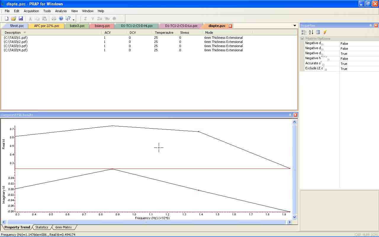
- Select 'OK'. The real and imaginary parts of the selected property will be plotted as a function of frequency.
- The results can be copied to the clipboard or printed on the PRAP printer..
One or more PRAP analyzed resonance files can be added to a PRAP compound file (of extension '.PZC'). By including resonance spectra analyzed at different temperature, the temperature dependence of material properties can be studied. The added resonance spectra should in general be acquired at the same DC bias voltage, temperature, etc.
To study the effect of temperature on the material properties;
- Open a new compound file with the 'New Compound File' command of the File menu.
- Using the File | Add Resonance File command or using the Edit | Paste command, add the spectra you wish to study.
- Ensure that each spectrum has been analyzed. You can do this by displaying each included resonance scan with the View | View Resonance Spectrum command.
- Selected the Analysis | Analysis Settings command.
- For the x-axis, select Temperature.
- For the y-axis, select the material property to be studied. The list of available properties is limited to those available from the analyzed resonance spectra included in the compound file.
- Select 'OK'. The real and imaginary parts of the selected property will be plotted as a function of temperature.
- The results can be copied to the clipboard or printed on the PRAP printer..
One or more PRAP analyzed resonance files can be added to a PRAP compound file (of extension '.PZC'). If each of these resonance files was acquired from samples with different applied DC bias voltages, or if each sample had a different thickness, each parameter can be plotted as a function of DC bias field.
Once a material property is plotted as a function of DC bias field, voltage, etc., a general, even, or odd polynomial can be fitted to the property using the 'Non-linear Regression' command of the Tools menu. The coefficients of the fitted polynomial can then be used in additional studies of your materials.
To study the effect of dc bias field on the material properties;
- Open a new compound file with the 'New Compound File' command of the File menu.
- Using the File | Add Resonance File command or using the Edit | Paste command, add the spectra you wish to study.
- Ensure that each spectrum has been analyzed. You can do this by displaying each included resonance scan with the View | View Resonance Spectrum command.
- Selected the Analysis | Analysis Settings command.
- For the x-axis, select DC Bias.
- For the y-axis, select the material property to be studied. The list of available properties is limited to those available from the analyzed resonance spectra included in the compound file.
- Select 'OK'. The real and imaginary parts of the selected property will be plotted as a function of dc bias.
- The results can be copied to the clipboard or printed on the PRAP printer..
One or more PRAP analyzed resonance files can be added to a PRAP compound file (of extension '.PZC'). By including resonance spectra analyzed at different times, the time dependence of material properties can be studied. The time since poling or since the application of a DC bias voltage could be studied. The added resonance spectra should in general be acquired at the same DC bias voltage and temperature.
To study the effect of frequency on the material properties;
- Open a new compound file with the 'New Compound File' command of the File menu.
- Using the File | Add Resonance File command or using the Edit | Paste command, add the spectra you wish to study.
- Ensure that each spectrum has been analyzed. You can do this by displaying each included resonance scan with the View | View Resonance Spectrum command.
- Selected the Analysis | Analysis Settings command.
- For the x-axis, select Time.
- For the y-axis, select the material property to be studied. The list of available properties is limited to those available from the analyzed resonance spectra included in the compound file.
- Select 'OK'. The real and imaginary parts of the selected property will be plotted as a function of time.
- The results can be copied to the clipboard or printed on the PRAP printer..
One or more PRAP analyzed resonance files can be added to a PRAP compound file (of extension '.PZC'). By including resonance spectra analyzed using different order resonance peaks, or by including the resonance spectra for samples having the same dimension aspect ratio and different resonance lengths, the frequency dependence of material properties can be studied. The added resonance spectra should in general be acquired at the same DC bias voltage, temperature, etc.
To study the effect of frequency on the material properties;
- Open a new compound file with the 'New Compound File' command of the File menu.
- Using the File | Add Resonance File command or using the Edit | Paste command, add the spectra you wish to study.
- Ensure that each spectrum has been analyzed. You can do this by displaying each included resonance scan with the View | View Resonance Spectrum command.
- Selected the Analysis | Analysis Settings command.
- For the x-axis, select Frequency.
- For the y-axis, select the material property to be studied. The list of available properties is limited to those available from the analyzed resonance spectra included in the compound file.
- Select 'OK'. The real and imaginary parts of the selected property will be plotted as a function of frequency.
- The results can be copied to the clipboard or printed on the PRAP printer..

One or more PRAP analyzed resonance files can be added to a PRAP compound file (of extension '.PZC'). If each of these resonance files is of different samples of the same material, the compound file will provide the average of the determined material properties along with the standard deviation of these properties given as the uncertainty in each property.
The average of each available property x is determined from;
\[ \bar{x} = \frac{1}{N} \sum_{i=1}^{N} x_i \]
where N is the number of available results for each property.
The standard deviation of each property is determined from;
\[ \sigma = \frac{1}{N} \sqrt{\sum_{i=1}^{N} \left( x_i - \bar{x} \right)^2 } \]
Note that each included analyzed resonance spectrum should generally be of the same resonance mode using the same order resonance peak. Other resonance modes and peaks can be used if frequency dispersion is to be ignored.
To study the statistics of your analysis results;
- Open a new compound file with the 'New Compound File' command of the File menu.
- Using the File | Add Resonance File command or using the Edit | Paste command, add the spectra you wish to study.
- Ensure that each spectrum has been analyzed. You can do this by displaying each included resonance scan with the View | View Resonance Spectrum command.
- The summary of statistical results is displayed in the Statistics tab of the Compound File Results View
- Statistical results can be copied to the clipboard or printed on the PRAP printer.
One or more PRAP analyzed resonance files can be added to a PRAP compound file (of extension '.PZC'). By combining the analysis results of the Basic Analysis Package 6mm length, thickness, radial extensional, and thickness shear resonance modes measured in the same material, 9 of the 10 independent properties in the [sE, d, εT] matrix of the reduced piezoelectric matrix for 6mm (C∞) materials are available. The use of the length-thickness extensional mode is optional. The undetermined property is sE13, and can be found from the following equation;
\[ \textbf s_{13}^E = \frac{- c_{13}^E s_{33}^E d_{13}}{e_{13} - d_{33} c_{13}^E } \]
where
\[ \textbf e_{13} = \frac{\epsilon_{33}^T - \epsilon_{33}^S - d_{33} e_{33}}{2 d_{13}} \]
\[ \textbf c_{13}^E = \frac{e_{33} - d_{33} c_{33}^E }{2 d_{13}} \]
Due to over-parameterization, frequency dispersion in material properties, and experimental errors, the analysis results from the thickness mode will not be identical to the [sE, d, εT] matrix transformed to the [cE, e, εS] matrix. The value for sE13 can be improved by transforming the completed matrix to the [cE, e, εS] matrix representation, comparing the corresponding cE33 to the value of cE33 determined directly from the resonance modes included in the compound file, and adjusting sE13 by the discrepancy. This procedure can then be repeated until results converge.
PRAP automates the above considerations in the 6mm Piezoelectric Matrix dialogue box. To construct the complete piezoelectric matrix;
- Open a new compound file with the 'New Compound File' command of the File menu.
- Using the File | Add Resonance File command or by pasting from the clipboard, add the spectra you wish to study.
- Ensure that each spectrum has been analyzed, and that samples from the 4 above-mentioned modes are included. You can ensure the spectra are analyzed by displaying each included resonance scan with the View | View Resonance Spectrum command.
- The signs of piezoelectric constants cannot be determined by resonance analysis. Assign the signs manually in the Properties view. In the same view the refinement options discussed above can be assigned.
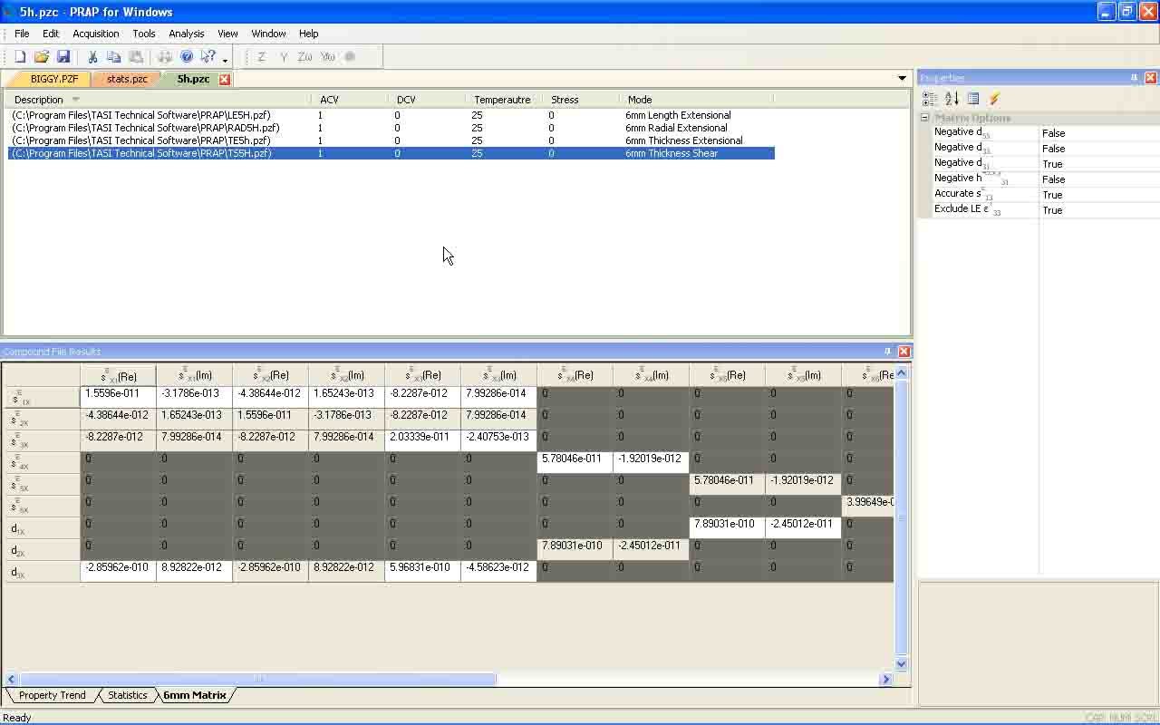
- The matrix representation displayed can be selected from the View menu.
- The determined matrix properties are displayed in the Compound File Results view by selecting the Matrix tab.
- Matrix results can be copied to the clipboard or printed on the PRAP printer.
Using the Rotated TE mode
Use of the LE mode is the usual way of computing the complete piezoelectric matrix. Because of the length of samples needed to induce the LE mode, they are difficult to pole and difficult to measure. In addition, properties determined from the LE mode are generally of a significantly lower frequency then the properties determined by the other three modes.
PRAP includes an additional TE mode where the direction of poling has been rotated 45° about the x or y axis. Use of this mode in the PRAP compound document permits the computation of the complete 6mm piezoelectric matrix of a material without use of the LE mode.
PRAP allows the generation of impedance frequency spectra for any mode or resonator supported by the software. To generate a new resonance spectrum from material properties:
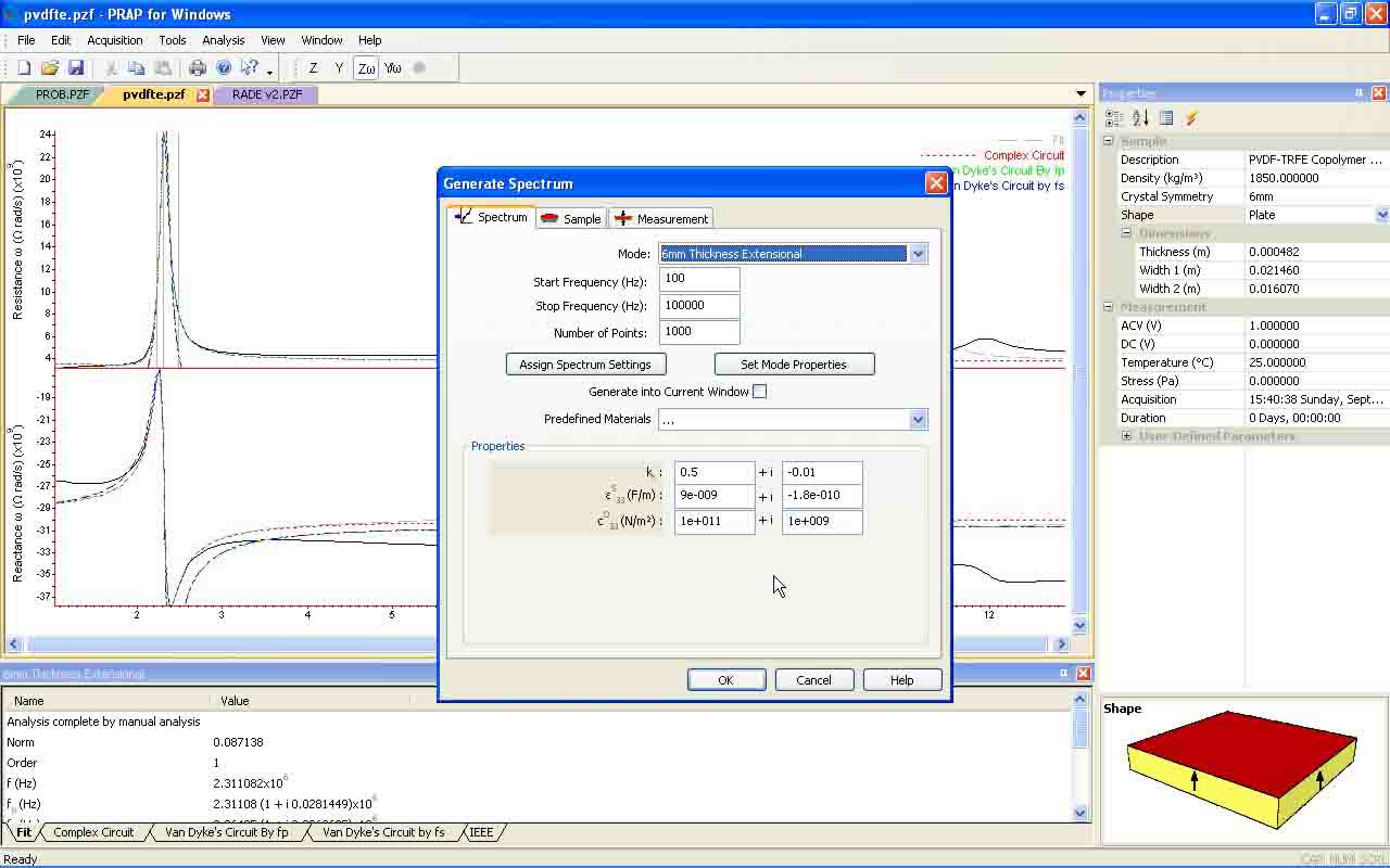
- Select the File | Generate command
- Select the mode and frequency of the spectrum to be generated.
- If a resonance spectrum is open in PRAP, the 'Assign Spectrum Settings' button will populate Sample and Measurement properties of the generated spectrum with those from the open existing spectrum.
- If a resonance spectrum is open in PRAP and the spectrum is analyzed with the same mode selected to be generated, the 'Set Mode Properties' will populated the material properties with those determined for the analyzed existing spectrum.
- if 'Generate into Current Window' is selected, the generated spectrum will be placed into the open spectrum as a fit. Otherwise the new spectrum will be generated into a new resonance spectrum file.
- Click on the Sample and Measurement tabs to assign the desired parameters for the generated spectrum.
- Press OK.
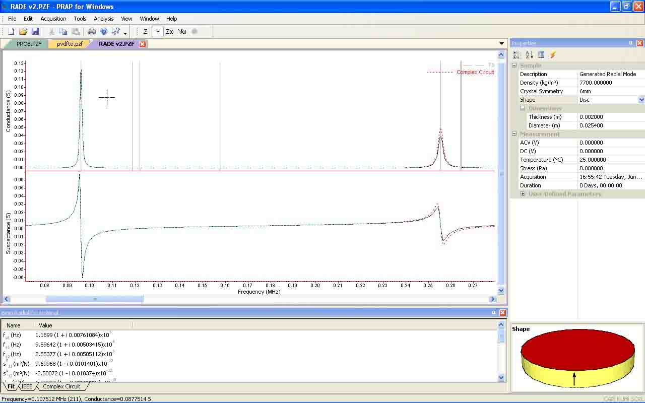
The radial mode is unusual in that it cannot be analyzed by non-linear regression, and analysis with the mouse requires use of the fundamental and 2nd order resonance peaks.
Analysis with the Mouse
- Select the 6mm Radial Extensional Mode from the Analysis menu
- Select Analysis | Analysis Settings
- Choose which analysis results are to be generated. Also select 'determine results for minimum norm' to choose whether the software will determine the best set of side-band frequencies, or whether it will have the user explicitly indicate these frequencies with the mouse. The Automatic fields determine the range of frequencies searched for a maximum upon selecting the Auto Analyze command. Press OK.
- Holding down the control key, click on the fundamental resonance peak. If the spectrum is not displayed in the Zω representation, the software will prompt you to make the transformation. If 'Locate nearest peak on click' was selected in the Analysis Settings dialog, the software will locate the maximum in the real part nearest the clicked point.
- If 'determine results for minimum norm' was selected in the Analysis Settings dialog the software will complete analysis of the radial mode. Otherwise holding down the control key you should select a point below the resonance peak with the left mouse button, clear of any 'bounce' in the spectrum and near the maximum in the G/ω representation.
- Holding down the control key, select a point above the resonance peak with the left mouse button. This should be near the minimum in the Xω curve of the spectrum at the fundamental resonance.
- Holding down the control key, select the 2nd order resonance peal. with the left mouse button. If 'Locate nearest peak on click' was selected in the Analysis Settings dialog, the software will locate the maximum in the real part nearest the clicked point.
- Holding down the control key you should select a point below the 2nd order resonance peak with the left mouse button, clear of any 'bounce' in the spectrum and near the maximum in the 2nd order peak G/ω representation.
- Holding down the control key, select a point above the 2nd order resonance peak with the left mouse button. This should be near the minimum in the Xω curve of the spectrum at the 2nd order resonance peak.
- Holding down the control key, click on the point used to evaluate permittivity with the left mouse button. This should in general be located between the fundamental and second order peak, or below the fundamental peak.
The options selected in the Analysis Settings dialog will dictate the results generated. Plotted results will have a legend on the right side of the graph.
The analysis of most resonance spectra are similar to the analysis of the TE mode. Depending on the mode, the Zω and G/ω representations may be reversed.
There are two fundamental ways of analyzing most resonance spectra. One is by non-linear regression, the other is with the mouse that utilizes a modified form of Smitt's method. The advantage of non-linear regression is that it provides an estimate of the uncertainty in the fitted properties. The disadvantage is that it is fitted over a range of frequency which becomes problematic when there is dispersion, and the method in general can suffer from degeneracies that can prevent convergence on a solution. The advantage of analysis with the mouse is that analysis can be isolated to the frequency region of the resonance peak, and it is possible to explicitly select which data points are used. Analysis with the mouse is the preferred form of analysis with PRAP (if it is available for the chosen resonance mode).
Non-linear Regression
- Select the 6mm Thickness Extensional Mode from the Analysis menu
- Select Analysis | Analysis Settings and then the Regression tab
- Ensure chi-squared and the minimal fractional change in chi squared are sufficiently small to ensure convergence. You may want to experiment with this for your spectra. You can also put restraints on the fitted material properties.
- Select Analysis | Fit Parameters. Specify the range of frequency to be fitted and the initial material property values. If analysis of the spectrum has already been done, the 'Use parameters of last fit will populate the properties with the previously determined properties of the mode.
- Select Fit. The fitted impedance curve should plotted as the parameters are updated.
Analysis with the Mouse
- Select the 6mm Thickness Extensional Mode from the Analysis menu
- Select Analysis | Analysis Settings
- Choose which analysis results are to be generated. Also select 'determine results for minimum norm' to choose whether the software will determine the best pair of side-band frequencies, or whether it will have the user explicitly indicate these frequencies with the mouse. The Automatic fields determine the range of frequencies searched for a maximum upon selecting the Auto Analyze command. Press OK.
- Holding down the control key, click on the resonance peak. If the spectrum is not displayed in the Zω representation, the software will prompt you to make the transformation. You should then enter the order of the selected resonance peak. The fundamental is order 1, etc. If 'Locate nearest peak on click' was selected in the Analysis Settings dialog, the software will locate the maximum in the real part nearest the clicked point.
- If 'determine results for minimum norm' was selected in the Analysis Settings dialog the software will complete analysis of the mode. Otherwise holding down the control key you should select a point below the resonance peak with the left mouse button, clear of any 'bounce' in the spectrum and near the maximum in the G/ω representation.
- Holding down the control key, select a point above the resonance peak with the left mouse button. This should be near the minimum in the Xω curve of the spectrum.
The options selected in the Analysis Settings dialog will dictate the results generated. Plotted results will have a legend on the right side of the graph.

The best way to obtain resonance spectra is by directly acquiring them from an impedance analyzer using the PRAP Data Acquisition interface. However it is also possible to import resonance spectra into PRAP by pasting from the clipboard or loading as a text file.
To proceed use the File | Save As command with an existing PZF file and select the PRAP Export Resonance File as the file type, or use the PRAP Edit | Copy command to copy an existing spectrum to the clipboard, then pasting it into a spreadsheet. This will ensure the correct fields are included. The fields should then be repopulated with details of the spectrum to be imported, and the resulting new file opened with the PRAP File | Open command (selecting the PRAP Export Resonance File as the file type) or pasting into PRAP with the Edit | Paste command. Fields in the import file should be tab-delimited.
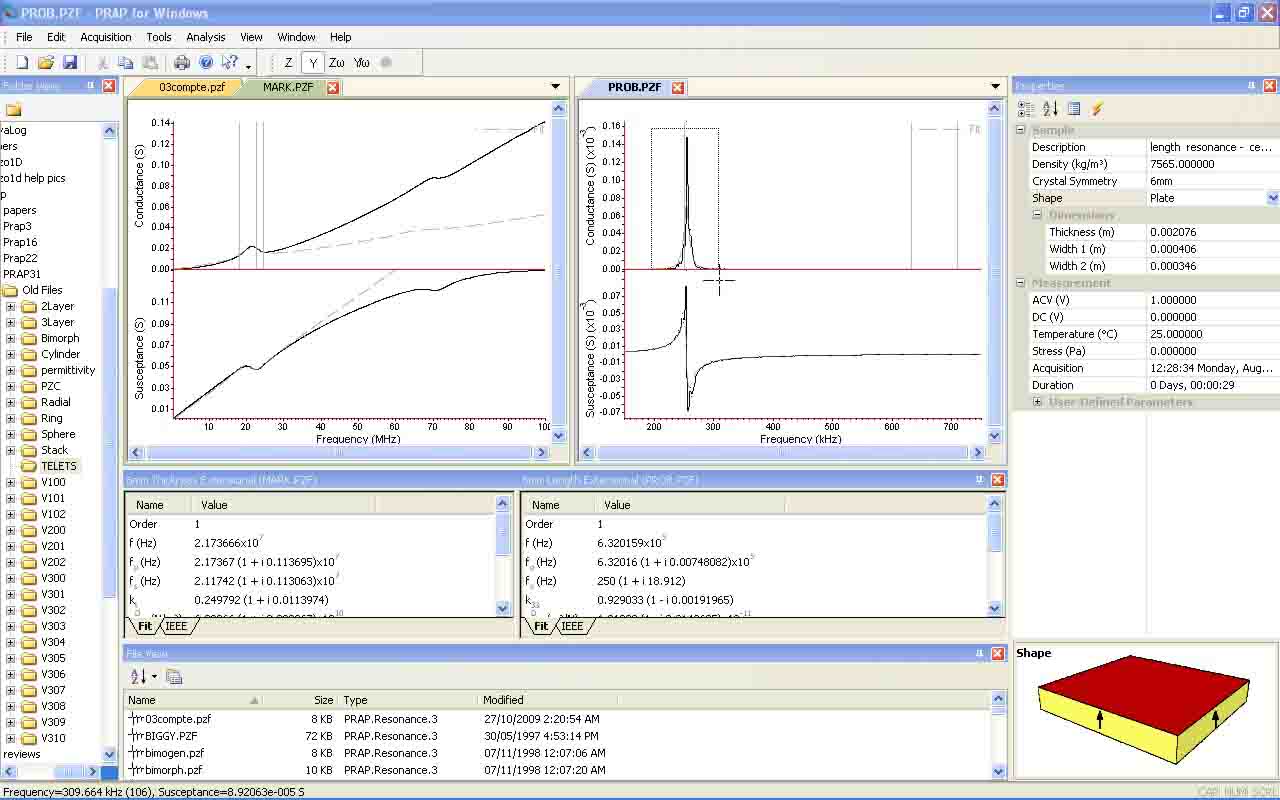
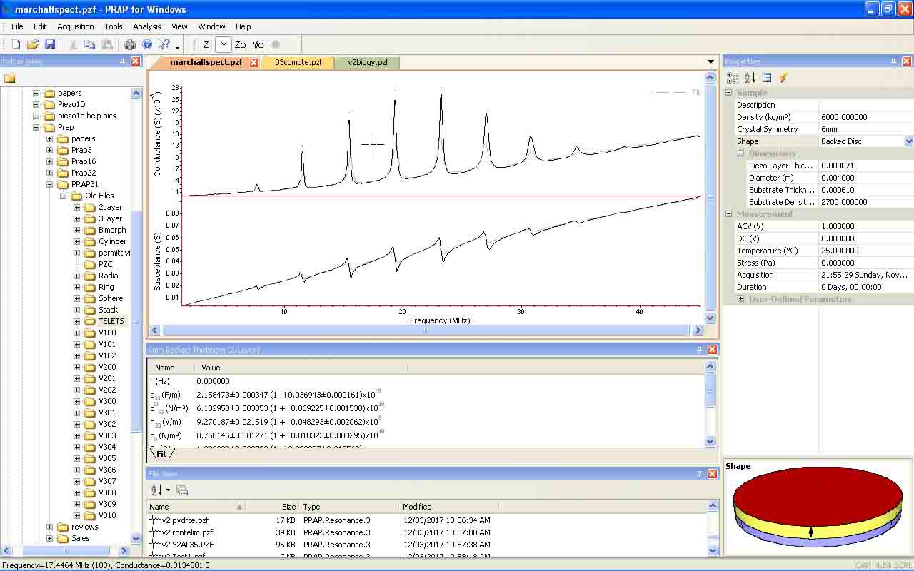
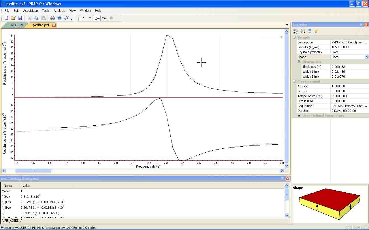
PRAP provides a graphical interface for loading, acquiring and analyzing resonance spectra. Each region of the interface is fully dockable meaning they can be re-arranged, opened or closed. The Folder View shows the folders of the file system while the File View shows the PRAP resonance and compound files of the file system. Resonance spectra and compound files are tabbed, and two files can be displayed side-by-side by dragging a tab off the tab frame. Analysis results are shown below the spectrum or compound file display in tabbed windows. The file properties are shown in the Properties View for the selected PRAP file.
Representation
The representation of a resonance spectrum can be controlled from the View menu where it can be displayed as a frequency spectrum or a locus plot. The representation can be selected between various types of impedance and admittance plots.
The View menu also allows control of the plotting of lines and data points, and whether the y-axis is plotted in a linear or logarithmic scale.
Ranging
The range of spectrum display can be controlled with the house. Clicking with the left mouse and dragging over the spectrum graph will allow a sub-range of the spectrum to be plotted. Clicking with the right mouse button steps out one 'zoom' level.
A license to use PRAP can be purchased which provides unlimited updates for one year. Within that year, 1-4 additional years of unlimited updates can be purchased. If updates are allowed to expire, an upgrade can be purchased. A licensed copy of PRAP can continue be used outside of the update period. In this case you would not be entitled to install new updates until an upgrade is purchased. Any valid PRAP license for any PRAP version is entitled to purchase an upgrade. See the following for details. All prices are in US dollars:
|
Item |
Price |
Benefit |
|
New License |
$5000.00 |
Unlimited updates for 1 year |
|
Upgrade to Existing License |
$2500.00 |
Unlimited updates for 1 year |
|
1 Year Updates |
$900.00 |
Extends unlimited updates for 1 year when purchased within update period |
|
2 Year Updates |
$1700.00 |
Extends unlimited updates for 2 years when purchased within update period |
|
3 Year Updates |
$2400.00 |
Extends unlimited updates for 3 years when purchased within update period |
|
4 Year Updates |
$3000.00 |
Extends unlimited updates for 4 years when purchased within update period |
Contact TASI Technical Software for additional information
PRAP Version 3.1
Released in 2017, Version 3.1 of PRAP is a completely re-designed application that continues to support the analytical capability of version 2.2. It is a 32bit Windows application that runs under Windows 7, 8.1 and 10. It will also continue to run on Windows XP systems. Most notable is that all acquisition and analysis modules of PRAP 2.2 are now included in the standard software license.
All releases of PRAP are available for download. Any of these revisions can be activated in Basic Mode. Basic Mode enables only the TE Resonance mode for analysis. With a Customer Number valid for the release date of each revision, the software can be fully enabled.
32 Bit acquisition may fail to load some instrument drivers
Changed export from 6 significant digits to 15 digits to embrace full resolution of double floating point
virtual destructor error
Import Settings would not save symmetry setting
Import of non-impedance data incorrectly labels axes as impedance
Added trap for failure to create Zw and Yw spectra in analysis
All Files now opens Import File for File Open
Changed to v143 VS toolset (previous was v141)
ResultStruct Mode changed from 64bit int under x64 to 32bit int
PZF thumbnail shell extension now working
Now prevent unsupported symmetry from being selected for sample
Spelling errors
Activation key modified so not corrupted by Windows Update
Added Edit : Properties to PZF file
Updated License file
Restricted Print and Copy for Basic version
Optimiser bug in compiler - 'volatile' hack prevented incorrect optimization
Added ODBC database connectivity to libraries
Import real and imaginary parse error
Lock process changed for analysis threads
Added Import Settings
Ability to specify how import spectra are read including encoding, header settings, and column content
Exported spectra incorrectly labeled Conductance as Admittance
Importing spectra sometimes attempted to read as UTF8 encoding
Added level of registry depth to instrument-specific settings
NI MX cards may not be detected if they did not have analog out
Cut and paste might set impedance values to 0 on import
Activation code could be corrupted. Installation of this revision will require re-activation
Newer Windows security could block installer from updating installation key. Installer now updates key
Acquisition time changed with each sample property change
Sample dimension changes in sample properties would not not change in resonance spectrum
Added relative permitivity to TELETS modes
Edited code to allow VS 2017 compile
Converted to 2017 source code libraries
Ended support for Win XP
import encoding could mistake UTF16 for UTF8
updated stack TE help
Last revision that will run under Windows XP
Error in activation xml file
TE and LE stack capacitance incorrectly labelled
g33eff in LE stack incorrectly labelled as g33
Bimorph k31 incorrectly labelled as k13
Ring k31 incorrectly labelled as k13
Cylinder k31 incorrectly labelled as k13
Too many ep31 properties in radial mode
Changes to database of the elements
Installer now resets installation code if does not match computer
Magnitude/Phase plots incorrectly transformed when acquired in this representation from impedance analyzer
Excluded poling for hp 4194a dc bias
Excluded poling for hp 4294a dc bias
Excluded poling for hp 4395a dc bias
Excluded poling for Tektronix 320 dc bias
PRAP programming incorrect property in phase acquisitions
VISAEventDev could miss an error in IsError
Added log scan to 4194a driver
Added deactivation to Help menu
Was not programming impedance analyzer signal strength
GPIB OpComplete bit not properly monitored
Refined sine correlation in use of signal generator and voltage measurement instrument
Extensive upgrade to use of signal generator and voltage measurement instrument
Removed Windows firewall settings from installer
TASI Visa incorrectly enumerating hardware resources
Inserted separator on Acquisition menu
Now disable DC Bias and Temperature scans if associated instruments are not assigned
Added HP4395a Network/Spectrum/Impedance Analyzer driver
Database of the elements moved to seperate module
Database of the elements now resizeable
Extensive work on new acquisition architecture
Added support for ProLogix USB-GPIB interface
Instrument drivers incorrectly loading string resources
Log plots not properly updated in status bar
Updated labeling for DisplaySettings
PRAP Appearance removed from Print Options
Code housekeeping with respect to database of materials
MaterialDB Compact option problem
Acquisition could crash if switching applications
Now Disable Assign Drivers and Configure Instruments of acquisition running
Added TwoLayer documentation
Added ThreeLayer documentation
Added cylinder documentation
Added ring documentation
Added sphere documentation
Updated acquisition of single spectrum including documentation
Added collection of spectra by dc bias with documentation
Added collection of spectra by temperature with documentation
Added collection of spectra by time with documentation
Radial mode was prompting for 1st peak order. Shouold always be 1st order
Exclusion of LE modes not working properly for 6mm and 4mm matrices
updated logic of piezo matrix signs and analysis options
Material database incorrectly displayed cE66 and cD66 for 4mm and 6mm symmetries
Material database incorrectly managing velocities
Added compact display mode for piezoelectric matrices compound file results
Added rotated TE mode 45 degrees about x or Y to 6mm piezo matrix
Added compact display mode for material database display
Added bimorph documentation
Some email calls for activation code would not work depending on system and email software installed
Added documentation for stack modes
Added customer number to email Activation email.
Added 'Add Resonance Spectrum' to PRAP Compound Document.
New server script on new server
Added PRAP compound files to windows shell
Added front end filtering of text files so encodings other than UTF-16 supported
Copy and paste of spectrum into spreadsheet could cause problems with spaces. Dimension names now single words
Compound files were not being serialized properly
Radial mode was not correctly reporting cE66
Copy/Export of material database now outputs according to selected matrix representation